3.3 Data from many Populations

Let us first create a directory specific for this tutorial:

mkdir atlas-tutorial_C
cd atlas-tutorial_C

3.3.1 Simulating Populations

In this tutorial, we will work with two populations, however, the same workflow can be used with more than two populations.

We will start by simulating two populations: The first one has 7 samples and a SFS with a theta of 0.001, the second one has 5 samples and a SFS with a theta of 0.005. This corresponds to the following site frequency spectrum file:

echo '#SHAPE=<15/11>
0.956105 0.009576 0.002592 0.003897 0.000011 0.001484 0.000339 0.000134 0.002077 0.000671 0.007219 0.000798 0.000000 0.000000 0.000000 0.000000 0.000000 0.000000 0.000000 0.000000 0.000000 0.000000 0.000827 0.000000 0.000000 0.000000 0.000000 0.000000 0.000000 0.000000 0.000000 0.000000 0.000000 0.000000 0.000000 0.000000 0.000000 0.000000 0.000000 0.000000 0.000000 0.000000 0.000000 0.000000 0.000474 0.000000 0.000000 0.000000 0.000000 0.000000 0.000000 0.000000 0.000000 0.000000 0.000000 0.001091 0.000000 0.000000 0.000000 0.000000 0.000000 0.000000 0.000000 0.000000 0.000000 0.000000 0.000000 0.000000 0.000000 0.000000 0.000000 0.000000 0.000000 0.000000 0.000000 0.000000 0.000000 0.000000 0.000000 0.000000 0.000000 0.000000 0.000000 0.000000 0.000000 0.000000 0.000000 0.000000 0.000000 0.000000 0.000000 0.000000 0.000000 0.000000 0.000000 0.000000 0.000000 0.000000 0.000000 0.001856 0.000000 0.000000 0.000000 0.000000 0.000000 0.000000 0.000000 0.000000 0.000000 0.000000 0.000322 0.000000 0.000000 0.000000 0.000000 0.000000 0.000000 0.000000 0.000000 0.000000 0.000000 0.000000 0.000000 0.000000 0.000000 0.000000 0.000000 0.000000 0.000000 0.000000 0.000000 0.000000 0.000000 0.000000 0.000000 0.000000 0.000000 0.000000 0.000000 0.000000 0.000000 0.000000 0.000000 0.000000 0.000000 0.000000 0.000000 0.000000 0.000000 0.000000 0.000000 0.000000 0.000000 0.000000 0.010526 0.000000 0.000000 0.000000 0.000000 0.000000 0.000000 0.000000 0.000000 0.000000 0.000000' > sfs.txt

Normally, we would start by simulating bam-files, estimating their errors, creating GLF files and finally estimating the major and minor alleles of the GLF-files. In this tutorial, we will use a shortcut, as Atlas can also simulate vcf-files directly:

atlas simulate --vcf --type SFS --sfs sfs.txt ---sampleSize 12

This creates the Variant Call Format file with major and minor alleles for all individuals. We can also create a matching sample file to tell us which sample belongs to which population.

echo 'IND POP
ind_0 pop_1
ind_1 pop_1
ind_2 pop_1
ind_3 pop_1
ind_4 pop_1
ind_5 pop_1
ind_6 pop_1
ind_7 pop_2
ind_8 pop_2
ind_9 pop_2
ind_10 pop_2
ind_11 pop_2' > samples.txt

3.3.2 Principal Component Analysis (PCA)

Before running a PCA, we first have to convert our VCF into another Variant Call Format, called Beagle. Because the PCA relies on information of variant sites only, we can filter sites with a very low minor allele frequency using the minMAF filter.

atlas convertVCF --format beagle --vcf ATLAS_simulations.vcf.gz --minMAF 0.05

To infer population structure with a PCA, we will use the tool PCAngsd. Please follow the following instructions to install it:

https://github.com/Rosemeis/pcangsd

We then run PCAngsd:

pcangsd --beagle ATLAS_simulations.beagle.gz

The results can be plotted in R (or Python, following the directions on https://github.com/Rosemeis/pcangsd):

C <- as.matrix(read.table("pcangsd.cov"))
e <- eigen(C)

samples <- read.table("samples.txt", header = T)
samples$POP <- factor(samples$POP)

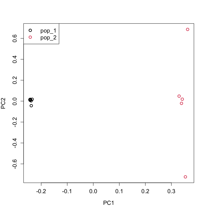
plot(e$vectors[,1:2], xlab="PC1", ylab="PC2", col = samples$POP)

Below an example of how that can look like - but note that the data you simulated may be a bit different.